Matching Data Between Two Sources Using Part of a String
The illustration below explains different scenarios to match data between two sources using part of a string.
Let us understand the requirement with an example. Click on each image if needed to open a larger view of the image.
The MASTER_LIST source contains a list of strings that need to be searched against the BANK_LIST source. The two sources are shown below.

For instance, if the search string is 'INDIA' in the MASTER_LIST source, the matching rows in the BANK_LIST source will be 'Indian Bank' and 'STATE BANK OF INDIA' since both bank names contain the string 'INDIA'. The resultant rows will be loaded into the BANK_MASTERtable as shown below.

The matching between the two sources should not be case-sensitive.
Scenario 1: When both the sources are relational tables and reside in the same database. The database for this example is Oracle.
The INSTR function returns the location of a substring in a string. If the INSTR function returns '0', it implies, the substring is not present in the original string. A SQL query that matches the data between the two sources is given below.
SELECT
mstr.master_id,
bank.bank_id,
bank.bank_name
FROM
master_list mstr, bank_list bank
WHERE
INSTR(bank.bank_name, mstr.search_string) > 0
The above query returns only one row as shown below.

The query should not be case-sensitive and it can be re-written as below by converting both the string (bank.bank_name) and the substring (mstr.search_string) to lower case. This query should be added to the Sql Query section in the Source Qualifier properties.
SELECT
mstr.master_id,
bank.bank_id,
bank.bank_name
FROM
master_list mstr, bank_list bank
WHERE
INSTR(LOWER(bank.bank_name), LOWER(mstr.search_string)) > 0
The mapping is a simple pass-through mapping as shown below.

The final output will be the same as shown in the BANK_MASTER table below with the desired four resultant rows.

Scenario 2: When both the sources are flat files or one source is a flat file and the other is a relational table.
In this example, both the sources are flat files. The mapping implementation is shown below.

After, the Source Qualifier transformations, create two expression transformations as shown above. Create two output ports MASTER_KEY and BANK_KEY in the expression transformations EXP_Master_List and EXP_Bank_List respectively and in the expression editor pass the integer value '1'. These values will serve as a dummy join to merge the rows from both the flat files in the joiner transformation.
In the joiner transformation, designate the MASTER_LIST source as the "Master" source since it has fewer rows as compared to the BANK_LIST source. The Joiner condition is shown below. The Join type is "Normal Join".

The joiner transformation essentially does a full outer join i.e. all the rows between the two sources are matched with each other. We need to select only those rows that meet the defined criteria. This is achieved by using a filter transformation with the Filter Condition as shown below.

Scenario 3: When both the sources are relational tables but reside in different databases.
A similar approach to Scenario 2 can be used in this case too, but it would mean joining all the rows between the two source tables in the joiner transformation. Rather we can issue a query to the BANK_LIST table similar to the query in Scenario 1 except that the query won't have the MASTER_LIST table since it is in a different database.
The SQL transformation can be used to process queries midstream and to get the matching rows from the BANK_LIST table.
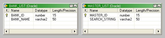
The source definitions for MASTER_LIST and BANK_LIST tables are shown below. Both the tables are in separate databases and there exists no DB links either between the two databases.

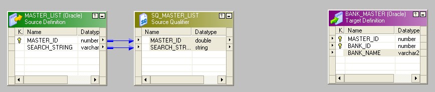
The BANK_MASTER target definition is shown below.

Create a new mapping. Drag the MASTER_LIST source definition and BANK_MASTER target definition into the Mapping Designer workspace as shown below.

Create a SQL transformation SQL_Get_Bank_Details as shown below. Click Create to proceed.

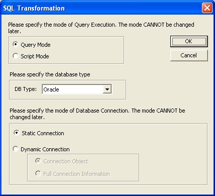
Proceed with the default settings as shown below. Click OK and Done to continue.
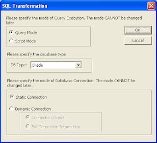
The SQL transformation needs to be run in the Query Mode since the SQL queries issued to the BANK_LIST table will be dynamic i.e. since the MASTER_LIST table contains two search strings 'INDIA' and 'AMERICA', two queries will be issued as given below.
SELECT BANK_ID, BANK_NAME
FROM
BANK_LIST
WHERE
INSTR(LOWER(BANK_NAME), LOWER('INDIA')) > 0;
SELECT BANK_ID, BANK_NAME
FROM
BANK_LIST
WHERE
INSTR(LOWER(BANK_NAME), LOWER('AMERICA')) > 0;
Drag the MASTER_ID and SEARCH_STRING ports from the Source Qualifier to the SQLtransformation as shown below.

Double click on the SQL transformation to edit it. Go to the SQL Ports tab. Uncheck the SEARCH_STRING as an output port since it is not required in the target as shown below. Only the MASTER_ID needs to be passed to the target, so it remains as an Input/Output port.
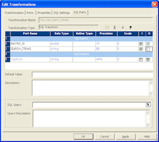
Add two SQL output ports BANK_ID and BANK_NAME as shown below ensuring that the correct Native Type and Precision are selected for each.

Next click on the section highlighted in red above to open the SQL Editor that will contain the SQL query that gets issued midstream. Type the query as shown below. Ensure that the order of the fields in the SELECT clause match the order of the SQL output ports.
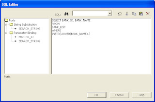
Now, since the 'SEARCH_STRING' needs to change dynamically as shown in the two queries above, we need to use String Substitution. Click on the SEARCH_STRING port below String Substitution to add it to the query as shown below.

Modify the query as shown below, so that it matches the above two queries that need to be issued to the BANK_LIST table.

Click OK to continue. Link the MASTER_ID_output, BANK_ID and BANK_NAME ports from the SQL transformation to the target definition. The complete mapping is shown below.

In the session task, mention the correct relational connections. A relational connection (Database_B) needs to be specified for the SQL transformation too. As shown below, the MASTER_LIST table is in Database_A, BANK_LIST table is in Database_B and BANK_MASTER target table is in Database_C.

Let us understand the requirement with an example. Click on each image if needed to open a larger view of the image.
The MASTER_LIST source contains a list of strings that need to be searched against the BANK_LIST source. The two sources are shown below.

For instance, if the search string is 'INDIA' in the MASTER_LIST source, the matching rows in the BANK_LIST source will be 'Indian Bank' and 'STATE BANK OF INDIA' since both bank names contain the string 'INDIA'. The resultant rows will be loaded into the BANK_MASTERtable as shown below.
The matching between the two sources should not be case-sensitive.
Scenario 1: When both the sources are relational tables and reside in the same database. The database for this example is Oracle.
The INSTR function returns the location of a substring in a string. If the INSTR function returns '0', it implies, the substring is not present in the original string. A SQL query that matches the data between the two sources is given below.
SELECT
mstr.master_id,
bank.bank_id,
bank.bank_name
FROM
master_list mstr, bank_list bank
WHERE
INSTR(bank.bank_name, mstr.search_string) > 0
The above query returns only one row as shown below.
The query should not be case-sensitive and it can be re-written as below by converting both the string (bank.bank_name) and the substring (mstr.search_string) to lower case. This query should be added to the Sql Query section in the Source Qualifier properties.
SELECT
mstr.master_id,
bank.bank_id,
bank.bank_name
FROM
master_list mstr, bank_list bank
WHERE
INSTR(LOWER(bank.bank_name), LOWER(mstr.search_string)) > 0
The mapping is a simple pass-through mapping as shown below.

The final output will be the same as shown in the BANK_MASTER table below with the desired four resultant rows.
Scenario 2: When both the sources are flat files or one source is a flat file and the other is a relational table.
In this example, both the sources are flat files. The mapping implementation is shown below.

After, the Source Qualifier transformations, create two expression transformations as shown above. Create two output ports MASTER_KEY and BANK_KEY in the expression transformations EXP_Master_List and EXP_Bank_List respectively and in the expression editor pass the integer value '1'. These values will serve as a dummy join to merge the rows from both the flat files in the joiner transformation.
In the joiner transformation, designate the MASTER_LIST source as the "Master" source since it has fewer rows as compared to the BANK_LIST source. The Joiner condition is shown below. The Join type is "Normal Join".

The joiner transformation essentially does a full outer join i.e. all the rows between the two sources are matched with each other. We need to select only those rows that meet the defined criteria. This is achieved by using a filter transformation with the Filter Condition as shown below.

Scenario 3: When both the sources are relational tables but reside in different databases.
A similar approach to Scenario 2 can be used in this case too, but it would mean joining all the rows between the two source tables in the joiner transformation. Rather we can issue a query to the BANK_LIST table similar to the query in Scenario 1 except that the query won't have the MASTER_LIST table since it is in a different database.
The SQL transformation can be used to process queries midstream and to get the matching rows from the BANK_LIST table.
The source definitions for MASTER_LIST and BANK_LIST tables are shown below. Both the tables are in separate databases and there exists no DB links either between the two databases.
The BANK_MASTER target definition is shown below.
Create a new mapping. Drag the MASTER_LIST source definition and BANK_MASTER target definition into the Mapping Designer workspace as shown below.
Create a SQL transformation SQL_Get_Bank_Details as shown below. Click Create to proceed.

Proceed with the default settings as shown below. Click OK and Done to continue.
The SQL transformation needs to be run in the Query Mode since the SQL queries issued to the BANK_LIST table will be dynamic i.e. since the MASTER_LIST table contains two search strings 'INDIA' and 'AMERICA', two queries will be issued as given below.
SELECT BANK_ID, BANK_NAME
FROM
BANK_LIST
WHERE
INSTR(LOWER(BANK_NAME), LOWER('INDIA')) > 0;
SELECT BANK_ID, BANK_NAME
FROM
BANK_LIST
WHERE
INSTR(LOWER(BANK_NAME), LOWER('AMERICA')) > 0;
Drag the MASTER_ID and SEARCH_STRING ports from the Source Qualifier to the SQLtransformation as shown below.

Double click on the SQL transformation to edit it. Go to the SQL Ports tab. Uncheck the SEARCH_STRING as an output port since it is not required in the target as shown below. Only the MASTER_ID needs to be passed to the target, so it remains as an Input/Output port.

Add two SQL output ports BANK_ID and BANK_NAME as shown below ensuring that the correct Native Type and Precision are selected for each.

Next click on the section highlighted in red above to open the SQL Editor that will contain the SQL query that gets issued midstream. Type the query as shown below. Ensure that the order of the fields in the SELECT clause match the order of the SQL output ports.

Now, since the 'SEARCH_STRING' needs to change dynamically as shown in the two queries above, we need to use String Substitution. Click on the SEARCH_STRING port below String Substitution to add it to the query as shown below.
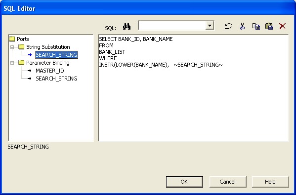
Modify the query as shown below, so that it matches the above two queries that need to be issued to the BANK_LIST table.

Click OK to continue. Link the MASTER_ID_output, BANK_ID and BANK_NAME ports from the SQL transformation to the target definition. The complete mapping is shown below.

In the session task, mention the correct relational connections. A relational connection (Database_B) needs to be specified for the SQL transformation too. As shown below, the MASTER_LIST table is in Database_A, BANK_LIST table is in Database_B and BANK_MASTER target table is in Database_C.